Algorithm for creating Charts in MS-Excel

1. Start
2. Click on Start Button à All Programs à MS Office à MS-Excel
3. Enter the heading for the program at A1 to D1 cells
4. Enter the given data from A3 to E8 cells, which is Year, Product-1, Product-2, Product-3 and Product-4 and corresponding data
5. Click on Insert menu Chart option, opens Chart wizard window which is of 4 steps
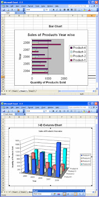
6. In Step 1 of 4, Select Chart type as Column and proper chart sub-type and click next button to proceed
7. In Step 2 of 4, Select Data range is A3 to E8 cells and select Series in as rows and give proper names for each series and Category X-axis labels as A3 row which is all headings and click next button
8. In Step 3 of 4, Type Chart title, X and Y axis titles, Axes, Gridlines, Legend, Data labels & Data tables as per your needs and click next button
9. In Step4 of 4, Place the prepared Chart which is ready to place it as an object in Sheet1 or in a new excel worksheet and Finish
10. Repeat Steps (5) thru (9) for 3D-Column and Bar Charts
11. Save the worksheet with proper name and Close the Excel worksheet
12. Stop